See the previous chapter…
- Course overview: goals and introduction
- Positions: latitude, longitude, nautical mile, scale, knots
- Nautical chart: coordinates, positions, courses, chart symbols, projections
- Compass: variation, deviation, true • magnetic • compass courses
- Plotting and piloting: LOPs, (running) fix, dead reckoning, leeway, CTS, CTW, COG
- Advanced piloting: double angle on the bow • four point • special angle fix, distance of horizon, dipping range, vertical sextant angle, radians, estimation of distances
- Astronomical origin of tides: diurnal, semi-diurnal, sysygy, spring, neap, axial tilt Earth, apsidal • nodal precession, declination Moon and Sun, elliptical orbits, lunar nodes
- Tides: tidal height prediction, chart datums, tidal curves, secondary ports
- Tidal streams and currents: diamonds, Course to Steer, Estimated Position
- Aids to navigation: buoys, leading lights, ranges, characteristics, visibility
- Lights and shapes: vessels sailing, anchoring, towing, fishing, NUC, RAM, dredging
7 – Tides & tidal height prediction
Chart datums
The depths and heights in the chart need a plane of reference: the chart datum (CD).
Depths are usually described with respect to low water reference planes (yielding lower charted depths, which are safer), and heights are shown with respect to high water reference planes (again, yielding lower vertical clearances on the chart, which are safer).
As such, the chance that the observed depth or vertical clearance beneath a bridge is smaller than the charted depth or height is rather small. The term clearance height is synonymous with vertical clearance.

Note, planes of reference are not exactly as shown above for all charts. Check for possible notes under the Chart Title. Hi-res image
“Observed depth” is synonymous with “depth of water”.
The image above demonstrates that:
- observed depth = charted depth + height of tide
- observed depth = height of tide − drying height
Soundings / charted depths
Charted depths or soundings are indicated on the charts by:
- contour depths (areas with different colour denoting a certain depth level)
- contour lines, e.g. —150—
- spot depths, e.g. 122
These soundings are reduced to the Chart Datum (CD), usually Lowest Astronomical Tide (LAT) in tidal waters.
A spot depth sounding like 35 indicates 3½ metres of water under LAT, whereas an underlined sounding like 04 indicates a height of 40 cm above LAT (or other CD), only the metres figure is underlined for drying areas.
From 0.1 to 20.9 metre depths are given in metres and decimetres.
From 21 to 31 in metres and half metres.
Greater depths are rounded down to the nearest safest metre, e.g. 32.7 metres is rounded down to 32 metres.
The geographical position of a spot depth sounding is the centre of the depth figure.
Nautical chart symbols for tidal levels & clearances
| CD | Chart Datum – Datum for sounding reduction |
| LAT | Lowest Astronomical Tide |
| HAT | Highest Astronomical Tide |
| MLW | Mean Low Water |
| MHW | Mean High Water |
| MSL | Mean Sea Level |
| MLWS | Mean Low Water Springs |
| MHWS | Mean High Water Springs |
| MLWN | Mean Low Water Neaps |
| MHWN | Mean High Water Neaps |
| MLLW | Mean Lower Low Water |
| MHHW | Mean Higher High Water |
| MHLW | Mean Higher Low Water |
| MLHW | Mean Lower High Water |
 |
Power lines Vertical clearance indicated between Pylons emphasised with |

|
Power lines with safety vertical clearance indicated between magenta |
 |
Overhead pipes with vertical clearance |
 |
Aerial cableway with vertical clearance |
 |
Telephone lines with vertical clearance |
 |
Fixed bridge with vertical clearance Horizontal clearance is charted with |
 |
Opening bridge with vertical clearance |
| Offshore position for which tidal levels are tabulated Magenta square and lower case lettering |
|
Currents and tidal streams
The term current is used to describe water movements which are generally
constant in direction, and are not dependent on astronomical conditions, hence non-tidal.
Currents occur as:
- The flow of river water in rivers and estuaries
- Permanent flows in other restricted waters eg İstanbul Boğazı (Bosporus, Turkey)
- Permanent or seasonal oceanic currents
- Temporary wind-induced currents
On the other hand, tidal streams are intrinsically linked with the vertical tidal (height of tide) changes in the tidal cycle, and come in two flavours:
- RectilinearRectilinear tidal streams are found in channels and estuaries, where the water can only flow in two opposite directions, often referred to as ebb and flood
- RotaryRotary tidal streams occur where the water is less restrained, allowing a continually changing direction rotating a full 360° in each tidal cycle. Although this gives rise to the term rotary, the flow is considerably stronger in two approximately opposite directions than in any others
Streams and currents are described by the direction towards it is running, contrary to wind directions . Also, only surface streams and currents are charted or tabulated for surface navigation.
In Chapter 8 – Tidal streams and currentsChapter 8 – Tidal streams and currents we will learn how to use tidal diamonds and tidal atlases to plot Course to Steer and Estimated Position diagrams.
Tidal levels in the chart
![]() Tidal level squares (see the example on the left for location “f”) are shown on nautical charts at locations where tidal levels, i.e. “heights” produces solely by tides, have been measured.
Tidal level squares (see the example on the left for location “f”) are shown on nautical charts at locations where tidal levels, i.e. “heights” produces solely by tides, have been measured.
Levels are included in the same chart and tabulated in a tidal level table, such as the three examples below.
All figures + data are for practice purposes only,
and not for navigational use.
There are different table variations for semi-diurnalsemi-diurnal, mixed semi-diurnalmixed semi-diurnal and diurnal tidesdiurnal tides.
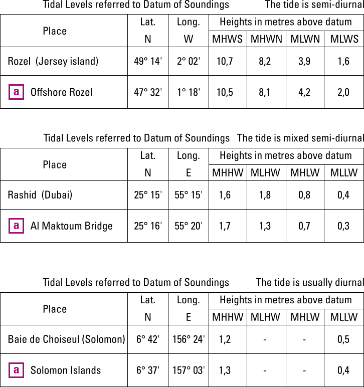
● SemiDiurnal Tides
● Mixed SemiDiurnal Tides
● Diurnal Tides
Note, that the coordinates don't give the leading zeros, especially the longitude positions, e.g. 2° W instead of 002° W, also see the style guide, in order to safe space and reduce chart clutter.
Tide tables
Tidal levels featured in the chart only give heights of tides, not times. Annual tide table books are used on board which specify the times of each HW and LW for each day of the year for standard ports (larger ports or reference ports). These publications should be used alongside the online tide resources, e.g. UK, USA, FR, NZL…
There are many tide table variations across countries and some mention times for high water only (view Cherbourg). More often the lunar phases 🌑︎ 🌒︎ 🌓︎ 🌔︎ 🌕︎ 🌖︎ 🌗︎ 🌘︎ 🌒︎, or neap and spring tides, or time difference between the two are added (i.e. Spring tide occurs two days after full and new moon.). Furthermore, dates to with daylight saving time applies can be conveniently indicated (view Dover).
Names of standard ports are usually written in bold letters.
The image below shows a portion of a typical tide table for any standard port. Note, that in (mixed) semi-diurnal tidessemi-diurnal tides, the tidal period is 12 hours and 25 minutes: from high tide to the next high tide. Therefore there are days, like Wednesday 2 January in this example, with just three entries.
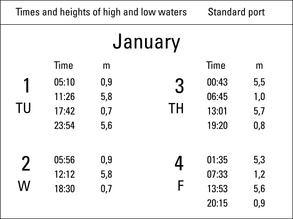
covering the first four days of January.
Times and heights of high waters and low waters are tabulated.
Times, time zones, UTC, GMT and Z
Times, in meteorology as well as nautical publications, are given using the 24-hour clock, based on the standard time of the country concerned. When a daylight-saving scheme is in operation, an hour has to be added to the time shown in the tide table or weather forecast in order to convert it to clock time.
The UK uses GMT (Greenwich Mean Time) and BST (British Summer Time in the summer months) as local time, but for instance France, Belgium and the Netherlands are one hour ahead, since located in the adjacent time zone; UTC+1. In order to convert a French tide table into GMT substract one hour. Most yachtsmen prefer to work in local time, rather than referring back to a home port's time zone.
GMT, CET (Central European Time; UTC+1) or for instance EST (Eastern Standard Time in the USA, New York; UTC-5) are time zones and based on the rotation of the earth.
UTC (Coordinated Universal Time) = Z (Zulu time) is not a time zone, rather is based on the caesium atomic clock. The UCT abbreviation was chosen as a compromise between English (CUT) and French speakers (TUC) and favours no particular language.
For navigational purposes both UTC and GMT (though now obsolete outside the UK) are regarded as interchangeable, yet UTC is recognized globally and the time zone offset should always be written as UTC±00.
Times should be written as 01:10 and not as 0110
Likewise, time differences as ±01:10 instead of ±0110
Notations with a colon (:) will also emphasise the correct meaning of 1 hour and 10 minutes (70 minutes) and not 110 minutes.
Note that Universal Time (UT) is a different standard.
Tidal curves
Tide tables give the heights for HW and LW each day, but to calculate the heights of tide between high and low waters, the standard ports have associated tidal curves published.It is far more likely that intermediate heights and times are required when entering / leaving a harbour, especially if there is a bar or sill (cill) to cross.
The tidal curve – together with the tide table – is used to find
Alongside the curve is a Mean Ranges box that states the average ranges of spring and neap tides.
The image below shows a typical tidal curve for a standard port with both spring tide and neap tide drawn. Here the mean range at spring tide is 4,9 m and and neap tide is 2,4 m.
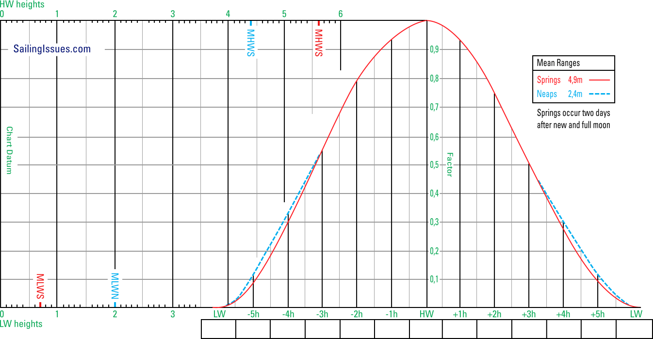
Both the spring and neap tide curves are drawn.
Mean ranges for springs and neaps are tabulated, plus moment of spring tide in the lunar month.
Using the tidal curve to find height of tide
In this example, the time we are interested in is 15:50 on 3 January of this year, see excerpt of the tide table below. On this day there are two low waters at 06:45 and 19:20 as well as two high waters at 00:43 and 13:01, a semidiurnal tidesemidiurnal tide therefore. These times are local times, and also no correction is needed for daylight saving time.
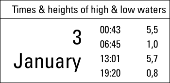
For 3 January the two HW and LW times and heights are given,
which values can be used combined with a tidal curve.
As we saw in Chapter 6 – Figure 6.12Figure 6.12, the range is “the difference between subsequent high and low waters levels”. Moreover, from the curve above we find that the mean range for springs is 4.9 m.
Therefore, the ranges indicate a near spring tide and an actual spring tide on this day:
5,5 − 1,0 = 4,5 (a near spring) and 5,7 − 0,8 = 4,9 (an actual spring).
Follow the six steps, in the filled-in tidal curve below, to learn how to find the tidal height at 15:50 at this standard port. To fill in a tidal curve either use pen + tracing paper, or a soft pencil.
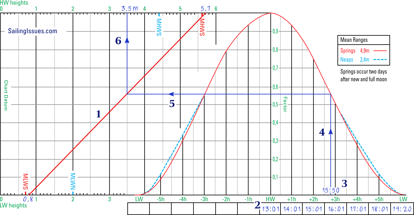
For 15:50 this means after the second HW, and therefore at spring.
- Draw the diagonal line between 0,8 and 5,7
The tide table for 3 January shows that it is spring tide, since 5,7 − 0,8 = 4,9 metres range, which is equal to the spring tide range indicated on the tidal curve.
Draw a line from the low water heights (at the bottom) to the high water heights (at the top). In this example the line is drawn in red to emphasize spring tide.
Certainly, the line starts close to the MLWS mark and ends close to the MHWS mark. - Fill in the times below the curve, starting with the nearest HW
Since 15:50 is after HW, start with adding 13:01 at HW and fill in the subsequent times for the hours after HW.
At LW the time of 19:20 illustrates that – although the curve uses the 12 hours – the tidal period is longer. Arguably, the following times should be added to the curve: 13:01 , 14:04 , 15:07 , 16:10 , 17:13 , 18:16 , 19:20, yet this practice is more complicated and would not make a significant difference. - Plot the time of 15:50
Using the added times after HW, plot the time of 15:50 on the horizontal axis of the curve. - Draw a vertical line from 15:50
End drawing the vertical line where it intersects with the red spring tide curve. Often the neap tide curve (dotted line) has a different shape. - Draw a horizontal line
End drawing the horizontal line where it intersects with the drawn diagonal. - Draw a vertical line to find the height of tide
From the intersection draw a vertical line (upwards is handier) and find the requested height of tide: 3,5 metres that corresponds with 15:50.
This answer can be verified using by the factor scale show above HW: 0,8 (start point of the range) + 0,56 (factor) * 4,9 (range) = 3,5 height of tide.
Using the tidal curve to find times
The tidal curve can also be used to find the times associated with a particular height of tide, for instance a 2 metres minimum height of tide that would allow passage across a bar.
In the example below six steps will lead from the desired height to specific times.
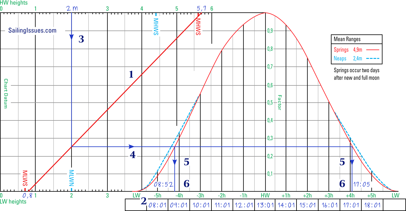
Starting from the desired level (2 metres in this example)
will result in a window of time (before and after HW)
when the tidal height is sufficient, i.e. more than 2 metres.
- Draw the diagonal line between 0,8 and 5,7
The tide table for 3 January shows that it is spring tide, since 5,7 − 0,8 = 4,9 metres range. Draw a line from the low water heights to the high water heights. In this example the line is drawn in red to emphasize spring tide. - Fill in the times below the curve
Start from HW and work towards both LWs. - Draw a vertical line from the height of 2 m
Start this line at the top scale at 2 m and end drawing where it intersects the diagonal. - Continue from there with a horizontal line
This horizontal line will intersect red spring tide curve twice. - Draw two vertical lines downwards from the two intersection points
One of these lines meets the time scale on the left side of HW, the other on the right side of HW. - Read off both times on the scale
In this example the height of tide will be 2 m at 08:52 and at 17:05. Between these times the height of tide will be larger and thus sufficient.
Secondary ports
Many of the more picturesque harbours and attractive anchorages visited by yachtspersons are classified as secondary ports. Since these smaller ports are of less commercial or military importance than standard ports neither tidal curves nor full tide tables are available.
Fortunately, official tide tables and almanacs have “tidal difference tables” which offer adjustments which – when applied to the times and heights of standard ports – result in the times and heights of the secondary port.
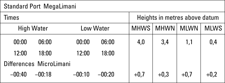
MicroLimani (litt. “small port” in Greek – “liman(i)” “port” in Turkish, Persian, etc., ultimately from Ancient Greek: λιμήν) as the secondary port, and MegaLimani as the standard port.
Eight differences are given: four minima and four maxima. For instance: the height difference at HW will be between the minimum +0,3 m and maximum +0,7 m.
The left section of the tidal difference table tells us:
- Time differences aka relative times; if HW MegaLimani is at
- 00:00 or at 12:00 then HW MicroLimani will be 40 minutes earlier
- 06:00 or at 18:00 then HW MicroLimani will be 18 minutes earlier
- 00:00 or at 12:00 then LW MicroLimani will be 10 minutes earlier
- 06:00 or at 18:00 then LW MicroLimani will be 20 minutes earlier
The right section of the tidal difference table tells us:
- Height differences; if HW MegaLimani is at
- 4,0 m (spring tide) then HW MicroLimani will be at 4,7 m
- 3,4 m (neap tide) then HW MicroLimani will be at 3,7 m
- 1,1 m (neap tide) then LW MicroLimani will be at 1,8 m
- 0,4 m (spring tide) then LW MicroLimani will be at 0,6 m
Time difference table: 4 vital details
By interpolating between the eight minima / maxima (four pairs) from the time difference table we can derive four vital details: the time differences of both HW and LW, and height differences of both HW and LW at the secondary port with respect to the standard port.
Secondary port examples
- Example 1 – finding HW time at MicroLimani secondary port
- Example 2 – finding LW time at Braye secondary port
- Example 3 – finding height of LW Braye secondary port
- Example 4 – finding HW time at Rye secondary port
- Example 5 – finding HW time at Les Sables d'Olonne
- Example 6 – finding height of HW Les Sables d'Olonne
Example 1 – Finding HW time at MicroLimani secondary port
In this example we will look at the afternoon of 16 May, for which the detailed tide table – see excerpt below – for the standard port of MegaLimani gives a HW 14:04 of 3,7 m and a subsequent LW 19:54 of 0,6 m.
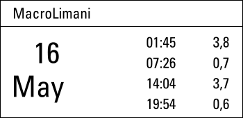
These HW / LW details – together with the tidal difference table – can be used to find HW / LW times and levels for a secondary port such as MicroLimani.
HW 14:04 is approximately 2 hours after 12:00 where the tidal difference table, see figure 7.8 shows −40 minutes, and is approximately 4 hours before 18:00 where the tidal difference table shows −18 minutes.
In these six hours the time difference decreases with 22 minutes in a linear fashion:
a 22/6 = 3,67 minute decrease for every hour.
Two hours and four minutes = 2,0667 hours; you can use a time to decimal calculator.
2,0667 × 3,67 = a decrease of 7,6 minutes,
resulting in −40 − −7,6 = approximately −32 minutes relative time.
Therefore, if HW MegaLimani is at 14:04 then HW MicroLimani will be at 13:32.
As an alternative to these calculations, you can draw the “Croc's teeth” or crocodile graph, see figure 7.10 below.
We will need (same as with the calculations) the secondary port's tidal difference table, and the standard port's tide table before plotting the graph.
Start by marking the two black axes: horizontally the time differences; and the angled axis with the times (or vice versa). Draw the long red line between the extremities of the axes. Then mark the time 14:04 along the time axis. Finally, draw – starting from 14:04 – an inner red line perpendicular to the larger red line.
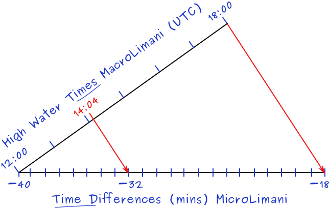
The axes should intersect at 12:00 and −40; the minima. Moreover, the outer diagonal should run between 18:00 and −18; the maxima.
In this example the relative time for HW at MicroLimani is −32 minutes. In case of daylight saving time (DST) the last step would be to add 1 hour.
There are four interpolations in total, and the three other interpolations for the secondary port – mutatis mutandis – will give us:
- height of tide at HW
- time of LW
- height of tide at LW
Use the tidal curve of the standard port for heights and times between LW and HW.
Example 2 – Finding LW time at Braye secondary port
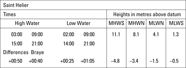
Jersey island's St Helier as standard port. Time and height differences with Braye (Alderney harbour) as secondary port.
To diversify globally, in this example the period ( . ) is used as a decimal separator, instead of the dot ( · ) or the comma ( , ).
Equivalent to the MicroLimani tidal difference table, the Braye table indicates that:
- if HW is at 03:00 or 15:00, it will be 50 mins later at Braye
- but if HW is at 09:00 or 21:00, it will be 40 mins later at Braye
- also when there is 11.1 m at HW at St Helier, there will be 4.8 m less at Braye, etc.
However, if high and low water are between these set times, we must interpolate between the “difference” amounts.
These HW / LW details – together with the tidal difference table – can be used to find HW / LW times and levels for the secondary port of Braye. Periods (.) used as decimal sign.
Note that Figures 7.13 and 7.14 are a rectangular variation on the (triangular) crocodile graph of figure 7.10, which further illustrates this interpolation method.
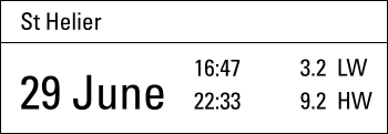
- Question: what is the time of LW Braye in the afternoon of 29 June when LW St Helier?
- Calculation: from Braye's tidal difference table, figure 7.11 we find the minima 14:00 [+00:25] and maxima 21:00 [+01:05]. Thus, the time difference increases in 7 hours from 25 to 65 mins, a total of 40 minutes, giving an hourly increase of 40/7 = 5.7 mins.
From the time table of St Helier, see figure 7.12, we find that afternoon LW is at 16:47
16:47 is 2 hrs and 47 mins after 1400 = 2.8 hrs
2.8 hrs × 5.7 mins = 16 mins
starting at the minimum of 25 time difference this is 25 + 16 = 41 minutes later than 16:47
Answer: time of LW Braye is 41 mins later than LW St Helier = 17:28 UCT. - Construction:
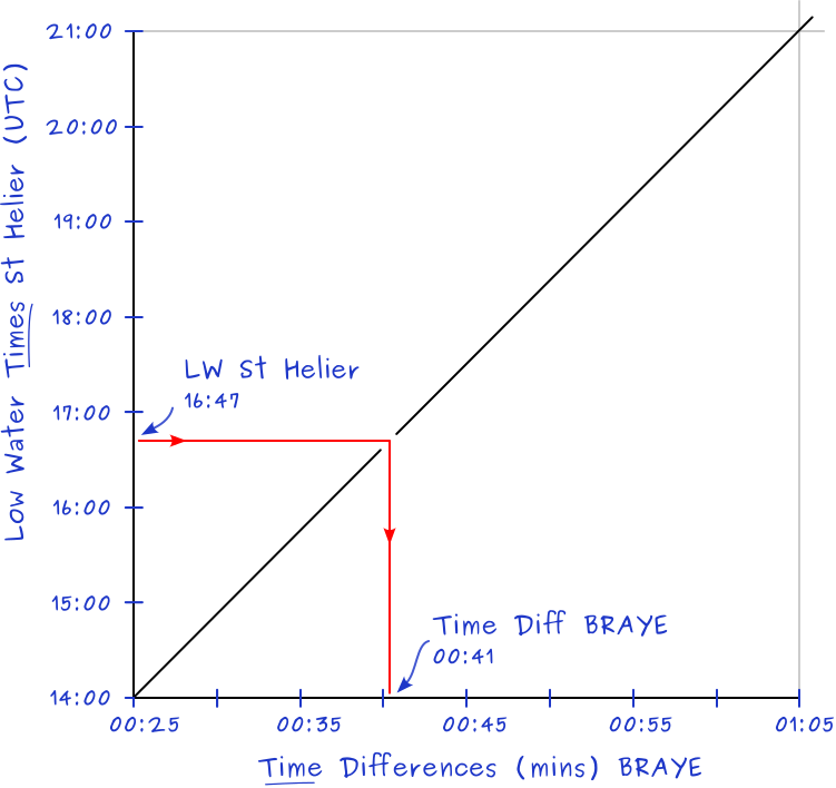
The two sets of values we need are the tidal difference table for the secondary port (Braye) and the LW time from time table standard port (St Helier).
The horizontal axis has the time differences in minutes between the ports.
The vertical axis has the times of LW at the standard port.
The axes should intersect at 14:00 and 00:25.
Alternatively draw the diagonal from 21:00 (top left) to 01:05 (bottom right). Then parallel to this line draw a short diagonal starting from 16:47. This means that the axes don't need to be perpendicular, and you can even switch the axes around.
Answer: Time of LW Braye = 16:47 + 00:40 = 17:27
Example 3 – Finding height of LW Braye secondary port
- Question: what is the height of LW at Braye when LW St Helier (standard port) is 3.2 m?
- Calculation: from Braye's tidal difference table, figure 7.11 we find spring 1.3 [−0.5] and neap 4.1 [−1.5]; there is a total LW height variance of 4.1 − 1.3 = 2.8 and
over these 2.8 metres a total change in height difference at Braye from −1.5 to −0.5 = −1.
The fraction of height is (3.2 − 1.3)/2.8 = 0.68
The lowest value of the height difference is −0.5.
Formula: fraction of height × total change in height difference + height difference lowest value = today's height difference at Braye
0.68 × −1 + −0.5 = −1.2
Answer: height of LW Braye = 3.2 + −1.2 = 2 m. - Construction:
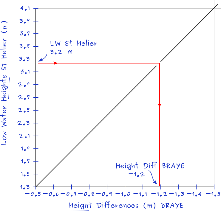
Spring 1.3 [−0.5] and neap 4.1 [−1.5] are from Braye's tidal difference table, see figure 7.11.The axes intersect at the minima 1.3 and −0.5. The LW Height axis ends at 4.1 and the Height Difference axis ends at −1.5.
3.2 m = height for LW St Helier from the tide table, see figure 7.12.
Either draw a line through 3.2 perpendicular to the line between 4.1 and −1.5, or draw the red lines as shown in this construction.
The result is a height difference of −1.2.
Therefore the LW height at Braye will be 1.2 less than 3.2 = 2 m.
Crocodile graph's shape and size are irrelevant
Note that the crocodile graphs – either rectangular or triangular – are based on linear changes.

In all three forms, “E” gives 5.75, see full screen image.
(a) The square graph is the easiest to comprehend, both the gray diagonals as the red lines can be used in this construction.
(b) The rectangular graph is stretched along the vertical axis without changing the outcome; the easiest to plot.
(c) The classic Croc's teeth graph is in fact the rhomboid shaped version of the square graph; only the “diagonal method” (in red) can be used.
The axes can be swapped, since mirrored in the black diagonal.
You can even change the plotting direction, so that minima become maxima, as long as this is done on both axes. The axis will then intersect at H and 10 rather than A and 0.
Example 4 – Finding HW time at Rye secondary port
Dover as standard port. Time high water differences with Rye as secondary port.
- Question: what time is HW Rye when HW Dover is 16:00?
- Calculation:
HW 16:00 Dover is 4 hours after 12:00 [+00:25], and
2 hours before 1800 [−00:50].
In these 6 hours the time difference is +25 − −50 = 75 mins.
Per hour a 75/6 = 12.5 mins decrease.
In four hours a 4 × 12.5 = 50 min decrease.
The −50 mins starts from +00:25 resulting in −00:25.
Answer: HW Rye is 25 mins earlier than 16:00 HW Dover at 15:35. - Construction: with time differences changing from − to + draw the crocodile graph as follows:
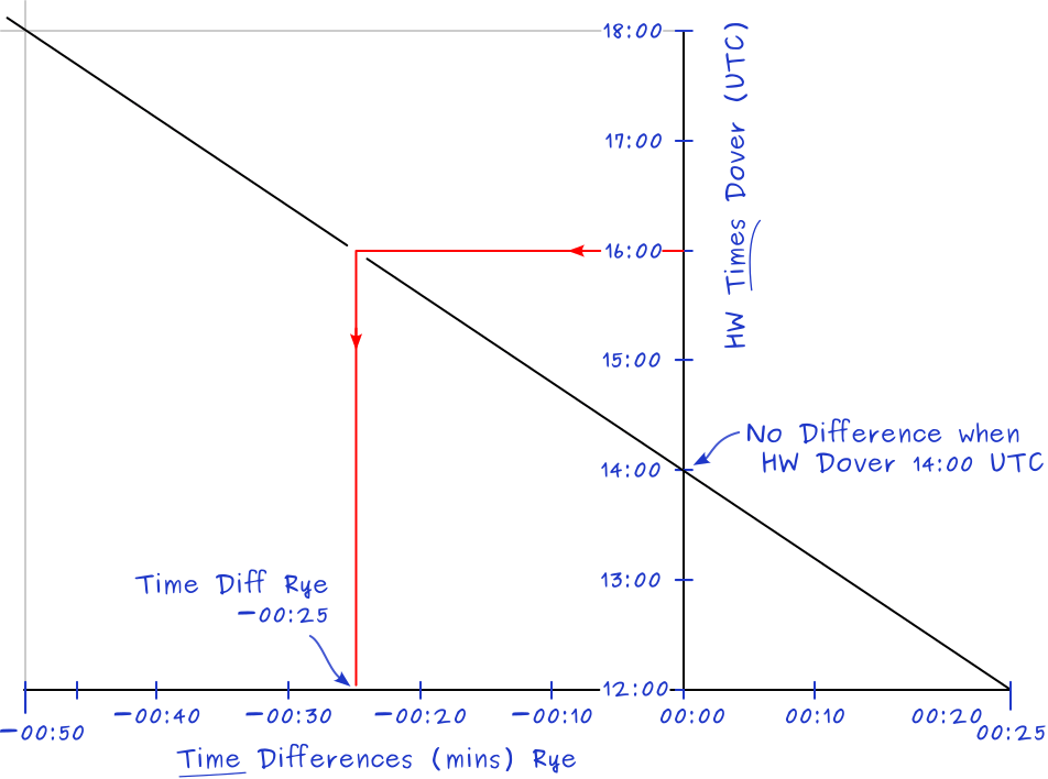
The horizontal axis has the Rye secondary port time differences with to the Dover standard port times (exaggerated differences).
Vertically the HW Dover times are plotted. Note that it is perfect alright to start the vertical axis from 00:25 (croc's teeth version) instead of 00:00, yet it is helpful to see instantly when the time difference is zero.
Example 5 – Finding HW time at Les Sables d'Olonne
With Brest on France's west coast as standard port and Les Sables d'Olonne as secondary port.
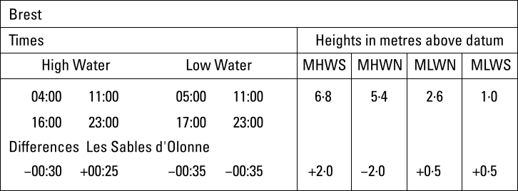
Time and height differences compared to Brest (standard port), Les Sables d'Olonne (secondary port).
To diversify globally, in this example the dot ( · ) is used as a decimal separator, instead of the period ( . ) or the comma ( , ).
These HW / LW details – together with the tidal difference table – can be used to find HW / LW times and levels for a secondary port such as Les Sables d'Olonne.
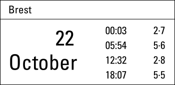
- Question: what time is HW Les Sables d'Olonne when HW Brest is 05:54?
- Calculation:
HW 05:54 Brest is 1.9 hours after 04:00 [−00:30], and
5.1 hours before 1100 [+00:25], see this useful time to decimal calculator.
In these 7 hours the total change in time difference is +25 − −30 = 55 mins,
which is per hour a 55/7 = 7.9 mins increase.
In 1.9 hours this is a 1.9 × 7.9 = 15 mins increase.
The +15 mins starts from −00:30 resulting in −00:15.
Answer: the time of HW Les Sables d'Olonne is 05:39, since 15 mins earlier than 05:54 HW Brest. - Construction:
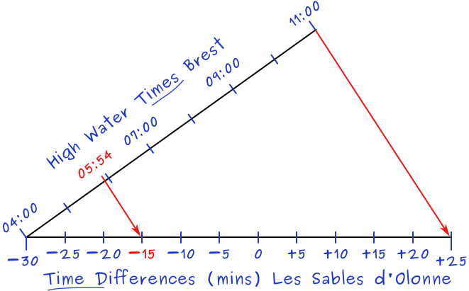
We find 04:00 [−00:30] and 1100 [+00:25] from the tidal difference table, see figure 7.18 with Brest as standard port.
The time differences at the secondary port are plotted here along the horizontal axis.
The axes intersect at the minima −30 and 04:00. The HW time axis ends at 11:00 and the Time Difference axis ends at +25 mins.
05:54 for HW Brest can be found in the tide table, see figure 7.19.
Draw the outer red line from 11:00 to +25 as shown, and subsequently a perpendicular line starting from 05:54.
The result is a time difference of −15, so HW Les Sables d'Olonne will be 15 minutes earlier than HW Brest at 05:39 UCT.
Example 6 – Finding height of HW at Les Sables d'Olonne
- Question: what is the height HW of Les Sables d'Olonne when height HW of Brest is 5·6 m?
- Calculation:
from Les Sables d'Olonne's tidal difference table, figure 7.18 we find spring 6·8 [+2·0] and neap 5·4 [−2·0]; there is a total HW height variance of 6·8 − 5·4 = 1·4 and
over these 1·4 metres a total change in height difference at Les Sables d'Olonne from 2 − −2 = 4.
The fraction of height is (5·6 − 5·4)/1·4 = 0·14 [a fraction or a percentage should always be a positive value: switch the numbers around when a negative value like 5·4 − 5·6 occurs]
The lowest value of the height difference is −2.
Formula: fraction of height × total change in height difference + height difference lowest value = today's height difference at secondary port
0·14 × 4 + −2 = −1·4
Answer: height of HW Les Sables d'Olonne = 5·6 + −1·4 = 4·2 m. - Construction:
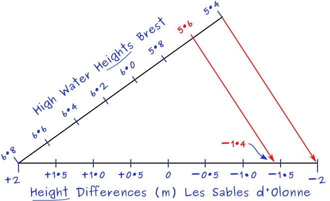
Spring 6·8 [+2·0] and neap 5·4 [−2·0] are from Les Sables d'Olonne's tidal difference table, see figure 7.18.
The axes intersect at the minima 6·8 and +2·0. The HW Heights axis ends at 5·4 and the Height Differences axis ends at −2·0.
5·6 m = height for HW Brest from the tide table, see figure 7.19.
Draw the inner red line from 5·6, and perpendicular to the line between 5·4 and −2·0.
The result is a height difference of −1·4.
So, the HW height at Les Sables d'Olonne will be 1·4 less than 5·6 = 4·2 m.
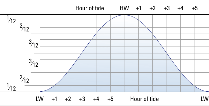
Rule of twelfths
The “rule of twelfths” is a simple method to – roughly – interpolate tidal heights between HW and LW without a tidal curve.
Tidal curves are mostly available for standard ports where sailing yachts would have ample water anyway; not in out of the way anchorages and smaller ports.
So how to determine the height of the tide (the tidal level) that is available to safely approach a depth restricted anchorage, harbour or pass over a sand bar?
All that is required to apply the rule of twelfths is the times and heights of both high or low water. From the difference between the tidal heights of high and low water the range can be calculated.
Figure 7.20 below shows an idealized semi-diurnal or mixed tidal cosine curve from HW to LW, i.e. a sinusoid with a period of 12 hours. Although simplified from 12 h 50 m this method will give acceptable results provided that the duration of rise or fall is between 5 and 7 hours.
- During the first hour after HW the water drops 1⁄12th of the full range.
- During the second hour an additional 2⁄12th
- During the third hour an additional 3⁄12th
- During the fourth hour an additional 3⁄12th
- During the fifth hour an additional 2⁄12th
- During the sixth hour an additional 1⁄12th, to a total of 12⁄12th (i.e. the full range)
To illustrate, two hours after HW the water has fallen 3⁄12th of the full range.
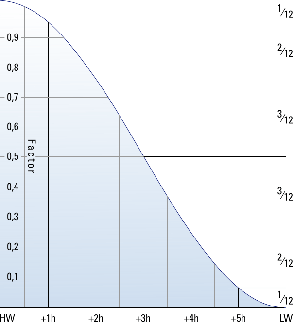
The tide doesn't rise or fall in a linear way, yet often follows a sinusoidal curve.
So, with the rule of twelfths we can estimate that e.g. after 4 hours the tide rises or falls by 9⁄12th of the range.
Some geographical locations do not have such a uniform curve. Very good examples of this can be found along the south coast of England, e.g. the Solent and Poole harbour have double high waters and Weymouth Bay has double low waters. In these instances, the rule of twelfths is ineffective and tabulated data online and in almanacs become vital.
Rule of seven
To interpolate between spring and neap tides we use the rule of seven.
Since the change from spring range to neap range can be assumed linear (instead of sinusoidal), each day the range changes with 1⁄7th of difference between the spring and neap ranges.
Hence, the daily change in range = (spring range − neap range)/7.
Beside interpolating for ranges, the rule of seven is also used to find rates of tidal streams between neap and spring rates, see tidal atlasestidal atlases.
Combining tidal predictions
Shown below is an example of a semi-diurnal tidal level table found in the chart – see the tidal levels section above, in this case for both the port of Dowes and for a position “b” just south of Dowes.
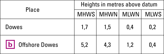
Tide table (or “chart”) showing minimal information on heights for the port of Dowes and for the approach of Dowes.
This succinct data only shows mean (i.e. “average”) high and low waters heights and also only for spring or neap tides. So, for this data to be useful, two further questions about relative times need to be answered:
- how many hours before or after HW?
- how many days before or after spring tide?
We need the times of high and low tides at the nearest standart port, as well as the relative times from the tidal difference table for Dowes.
Once both times are known, the two following problems can be solved.
Namely, finding height of tide at a particular location at a particular time to:
1. Shoal problem
A standard navigational problem is to establish whether the height of tide allows the crossing of a shoal, or, if not, the time at which the tide will have risen sufficiently.
The shoal offshore Dowes "b" has a charted depth of 1 meter, which needs to be crossed at about 15:00 hours with a yacht with a draft of 2 m.
From the nautical almanac we can find that at the nearest standard port HW occurs at 03:18 and 15:53 and LW at 09:45 and 22:03.
Also, HW occurs at Dowes one hour later, which is therefore at 16:53.
Spring tide is due in two days.
- Today's range, from figure 7.12 we get a spring range = 5,2 − 0,4 = 4,8 m and a neap range = 4,3 − 1,2 = 3,1 m.
Via the rule of seven we find out that today the range is:
spring range − 2 days × (spring range − neap range)/7 = today's range
4,8 − 2 × (4,8 − 3,1)/7
4,8 − 2 × 1,7/7
4,8 − 2 × 0,24
4,8 − 0,48 = 4,3 m, and verify that today's range is lower than spring range. - Today's HW height is likewise two days before spring.
Again from figure 7.12 we get a spring HW of 5,2 m and a neap HW of 4,3 m, leading to:
spring HW − 2 days × (spring HW − neap HW)/7 = today's HW height
5,3 − 2 days × (5,2 − 4,3)/7
5,3 − 2 × 0,9/7
5,3 − 2 × 0,13
5,3 − 0,26 = 5,0 m, and verify that today's HW height is lower than at spring. - Our intended crossing at 15:00 is nearly 2 hours before HW Dowes 16:53.
Via the rule of twelfths, and combining the two results above, we can find the tidal height of 15:00 today:
today's HW height − (1⁄12 + 2⁄12) × today's range = height at 15:00
5,0 − 3⁄12 × 4,3
5,0 − 1,08 = 3,9 m.
After three interpolations we derive the tidal height at 15:00 hours at our secondary port. Considering the charted depth of 1 meter this leads to an observed depth of 4,9 meters, sufficient for our draft of 2 meters.
Water under the keel
It is good practice to have at least 1 meter under the keel, and don't forget to include wave / swell height.
2. Bridge problem
Power lines or bridges have their clearance heights charted with respect to another chart datum than LAT. Often, Highest Astronomical Tide (HAT) is used as the reference plane for vertical clearances, see figure 7.1.
HAT – convert HW to HAT, obviously HAT is higher than Mean High Water Spring.
Note that HAT and LAT are “astronomical” and therefore not the extreme levels which can be reached as storm surges may cause considerably higher and lower levels to occur (ie. not taking into account air pressure or wind). If MHWS to HAT details are not available you should add an extra 10%.
You can find the height of HAT above Chart Datum for standard ports, either on a table of levels on your chart, or in the almanac tide tables for that port (e.g. see the tidal levels of New Zealand's standard ports.
An example: above our shoal hangs the “Dowes bridge” and at 15:00 hours we would like to pass under this bridge, which has a charted vertical clearance of 20 meters to HW.
Our mast height is 23 meters from the waterline. In the shoal example above we found that the water height was 1,1 meters below HW level at that time. Obviously, we will have to wait!
So, at what time will we be able to pass under this bridge?
The water height must be 3 meters lower than HW level (5,0 m). That is almost 9/12 of the range (4,3 m) indicating four hours after HW.
1/12 + 2/12 + 3/12 + 3/12 = 9/12.
Conclusion, we will have to wait at least six hours in total, since 15:00 is two hours before HW.
Weather influences on tides
The astronomical factors (Moon, Sun, axial tilt, orbital tilt… see chapter 6 – The astronomical origins of tideschapter 6 – The astronomical origins of tides) result in very accurate tide predictions, and even for complex coastal situations with estuaries and islands, local calculations and observations still give tidal levels with a precision of minutes in time and within a decimetre in height.
For standard ports, shipping lanes, etc. these predictions are published on nautical charts, in tidal atlases, (online) tide tables and numerous apps.
Yet, local wind and weather patterns will also affect tides and are obviously not taken into account in these publications.
- Offshore winds can move water away from coastlines, exaggerating low tide exposures.
- Onshore winds may act to pile up water onto the shoreline, sometimes even eliminating low tide exposures. With a prolonged Bft 5 blowing onshore a temporary wind-induced current can raise the sea level by 2 decimetres.
- High-pressure systems can depress sea levels, leading to clear sunny days with exceptionally low tides.
- Low-pressure systems that contribute to cloudy, rainy conditions typically are associated with tides than are much higher than predicted. Every extra 11 mbar of pressure (Greek: βάρος baros, meaning “weight”) can affect a change of 1 decimetre.
The combined effect of wind and barometric pressure typically produces variations of roughly ± 2 decimetres in height and ± 10 minutes in time, yet with extreme northerlies blowing down into the funnel-shaped North Sea, for instance, a raise of 2 metres and with a storm tide even 5 metres is possible.
Although tidal calculations should be carried out as meticulously as possible, their accuracy should not be relied on. Furthermore, even a small distance away from the actual position of tabulated tidal data could mean significant differences in times and tidal heights, set and rate.
Overview
- Tide: The vertical rise and fall of the surface of a body of water caused primarily by the differences in gravitational attraction of the moon, and to a lesser extent the sun, upon different parts of the earth when the positions of the moon and sun change with respect to the earth.
- Spring Tide: The tidal effect of the sun and the moon acting in concert twice a month, when the sun, earth and moon are all in a straight line (full moon or new moon). The range of tide is larger than average.
- Neap Tide: This opposite effect occurs when the moon is at right angles to the earth-sun line (first or last quarter). The range of tide is smaller than average.
- Range: The vertical difference between the high and low tide water levels during one tidal cycle.
- Tidal Day: 24 hours and 50 minutes. The moon orbits the earth once earth month, and the earth rotates (in the same direction as the moon's orbit) on its axis once every 24 hours.
- Tidal Cycle: A successive high and low tide.
- Semi-diurnal Tide: The most common tidal pattern, featuring two highs and two lows each day, with minimal variation in the height of successive high or low waters.
- Diurnal Tide: Only a single high and a single low during each tidal day; successive high and low waters do not vary by a great deal. Gulf of Mexico, Java Sea and in the Tonkin Gulf.
- Mixed Tide: Characterized by wide variation in heights of successive high and low waters, and by longer tide cycles than those of the semidiurnal cycle. U.S. Pacific coast and many Pacific islands.
- Chart Datum or Tidal reference planes: These fictitious planes are used as the sounding datum for the tidal heights.
- Drying Height: Clearance in meters (or feet in old charts) above the chart datum.
- Charted Depth: Clearance in meters (or feet in old charts) below the chart datum.
- Observed Depth: Height of tide + charted depth: the actual depth in meters.
- Height of light: The height of light above the bottom of its structure.
- Elevation: The height of the light above the chart datum.
- Rule of Twelve: Assuming a tidal curve to be a perfect sinusoid with a period of 12 hours. The height changes over the full range in the six hours between HW and LW with the following fractions during each respective hour: 1⁄12th ; 2⁄12th ; 3⁄12th ; 3⁄12th ; 2⁄12th ; 1⁄12th of the full range.
Rule of twelfths with tidal heights. - Rule of Seven: The change from spring range to neap range can be assumed linear, each day the range changes with 1⁄7th of difference between the spring and neap ranges. Hence, the daily change in range = (spring range − neap range)/7. The rule of seven is also used to find rates of tidal streams between neap and spring rates.
- Chart Datum or Tidal reference planes: These fictitious planes are used as the sounding datum for the tidal heights.
- Drying Height: Clearance in meters (or feet in old charts) above the chart datum.
- Charted Depth: Clearance in meters (or feet in old charts) below the chart datum.
- Observed Depth: Height of tide + charted depth: the actual depth in meters.
- Height of light: The height of light above the bottom of its structure.
- Elevation: The height of the light above the chart datum.
- Rule of Twelve: Assuming a tidal curve to be a perfect sinusoid with a period of 12 hours. The height changes over the full range in the six hours between HW and LW with the following fractions during each respective hour: 1/12 2/12 3/12 3/12 2/12 1/12.
- Rule of Seven: The change from spring range to neap range can be assumed linear, each day the range changes with 1/7th of difference between the spring and neap ranges. Hence, the daily change in range = (spring range − neap range)/7.
See the next chapter…
- Course overview: goals and introduction
- Positions: latitude, longitude, nautical mile, scale, knots
- Nautical chart: coordinates, positions, courses, chart symbols, projections
- Compass: variation, deviation, true • magnetic • compass courses
- Plotting and piloting: LOPs, (running) fix, dead reckoning, leeway, CTS, CTW, COG
- Advanced piloting: double angle on the bow • four point • special angle fix, distance of horizon, dipping range, vertical sextant angle, radians, estimation of distances
- Astronomical origin of tides: diurnal, semi-diurnal, sysygy, spring, neap, axial tilt Earth, apsidal • nodal precession, declination Moon and Sun, elliptical orbits, lunar nodes
- Tides: tidal height prediction, chart datums, tidal curves, secondary ports
- Tidal streams and currents: diamonds, Course to Steer, Estimated Position
- Aids to navigation: buoys, leading lights, ranges, characteristics, visibility
- Lights and shapes: vessels sailing, anchoring, towing, fishing, NUC, RAM, dredging
Also you can download the exercises + answers PDF ![]()